Visualizations with statistical details: The 'ggstatsplot' approach

Indrajeet Patil

doi:10.21105/joss.03167

Lifecycle:

The function gghistostats can be used for data exploration and to provide an easy way to make publication-ready histograms with appropriate and selected statistical details embedded in the plot itself. In this vignette we will explore several examples of how to use it.

Some instances where you would want to use gghistostats-

to inspect distribution of a continuous variable
to test if the mean of a sample variable is different from a specified value (population parameter)

Statistical analysis with `gghistostats`

Let’s begin with a very simple example from the psych package (psych::sat.act), a sample of 700 self-reported scores on the SAT Verbal, SAT Quantitative and ACT tests. ACT composite scores may range from 1 - 36. National norms have a mean of 20.

library(psych)

dplyr::glimpse(psych::sat.act)
#> Rows: 700
#> Columns: 6
#> $ gender    <int> 2, 2, 2, 1, 1, 1, 2, 1, 2, 2, 1, 2, 1, 2, 2, 2, 2, 2, 1, 2, …
#> $ education <int> 3, 3, 3, 4, 2, 5, 5, 3, 4, 5, 3, 4, 4, 4, 3, 4, 3, 4, 4, 4, …
#> $ age       <int> 19, 23, 20, 27, 33, 26, 30, 19, 23, 40, 23, 34, 32, 41, 20, …
#> $ ACT       <int> 24, 35, 21, 26, 31, 28, 36, 22, 22, 35, 32, 29, 21, 35, 27, …
#> $ SATV      <int> 500, 600, 480, 550, 600, 640, 610, 520, 400, 730, 760, 710, …
#> $ SATQ      <int> 500, 500, 470, 520, 550, 640, 500, 560, 600, 800, 710, 600, …

By default, gghistostats chooses a binwidth of (max(x) - min(x)) / sqrt(N). You should always check this value and explore multiple widths (via the binwidth argument) to find the best to illustrate the stories in your data since histograms are sensitive to binwidth. If you want a simple histogram without any statistical details, set results.subtitle = FALSE (and centrality.plotting = FALSE to also remove the centrality line).

Let’s test the hypothesis that our sample mean is the same as our national population mean of 20 using a parametric one sample t-test (the default type = "parametric").

gghistostats(
  data = psych::sat.act, ## data from which variable is to be taken
  x = ACT, ## numeric variable
  xlab = "ACT Score", ## x-axis label
  title = "Distribution of ACT Scores", ## title for the plot
  test.value = 20, ## test value
  caption = "Data courtesy of: SAPA project (https://sapa-project.org)"
)

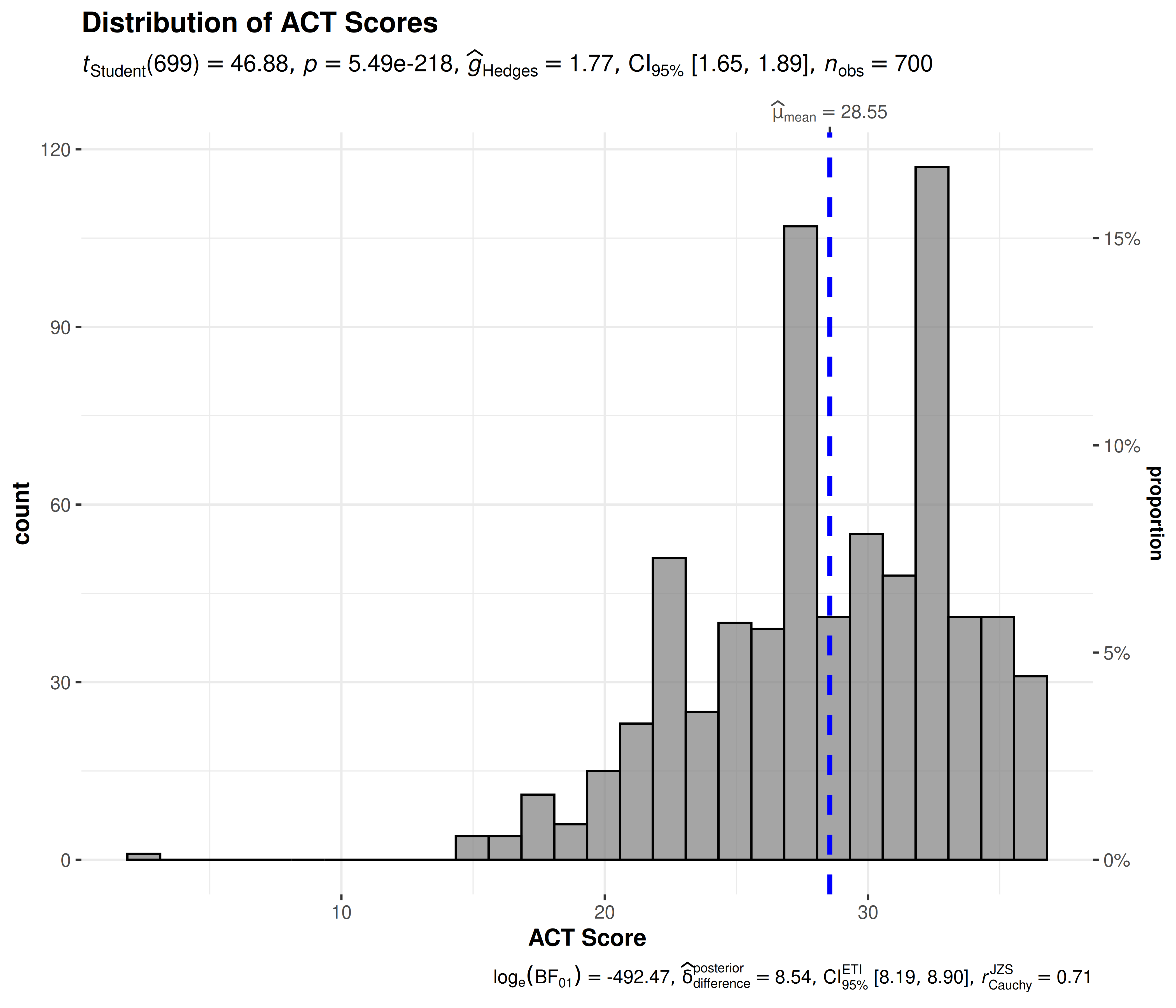
The caption reports $\log_{e}(BF_{01})$ . A negative value favors the alternative model; a positive value favors the null model. This compares how well the models predict the data, rather than giving the probability that a hypothesis is true. See Interpretation of Bayes Factors for details.

Grouped analysis with `grouped_gghistostats`

What if we want to do the same analysis separately for each gender? ggstatsplot provides a special helper function for such instances: grouped_gghistostats. This is merely a wrapper function around combine_plots. It applies gghistostats across all levels of a specified grouping variable and then combines the individual plots into a single plot. Note that the grouping variable can be anything: conditions in a given study, groups in a study sample, different studies, etc.

Let’s see how we can use this function to apply gghistostats to accomplish our task.

grouped_gghistostats(
  ## arguments relevant for gghistostats
  data = psych::sat.act,
  x = ACT, ## same outcome variable
  xlab = "ACT Score",
  grouping.var = gender, ## grouping variable males = 1, females = 2
  type = "robust", ## robust test: bootstrap-t test for one-sample trimmed mean
  test.value = 20, ## test value against which sample trimmed mean is to be compared
  centrality.line.args = list(color = "#D55E00", linetype = "dashed"),
  ## arguments relevant for combine_plots
  annotation.args = list(
    title = "Distribution of ACT scores across genders",
    caption = "Data courtesy of: SAPA project (https://sapa-project.org)"
  ),
  plotgrid.args = list(nrow = 2L)
)

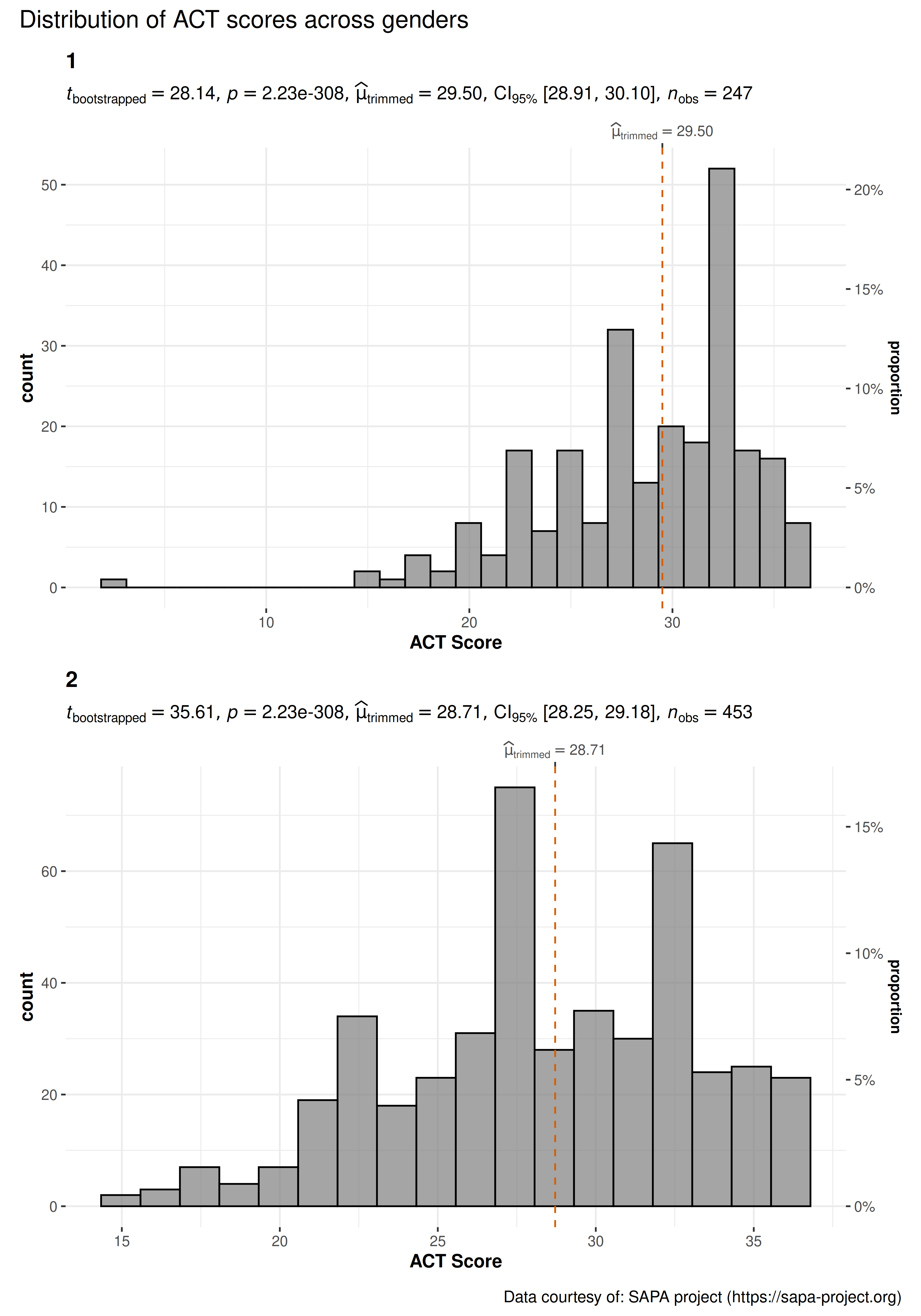
As can be seen from these plots, the trimmed mean is much higher than the national norm. Additionally, we see the benefits of plotting this data separately for each gender. We can see the differences in distributions.

Grouped analysis with `{purrr}`

For group-specific arguments or multiple grouping variables, see the programmatic plotting article. It explains how to split the data, customize each call, and combine the resulting plots.

Summary of graphics and tests

graphical element	`geom` used	argument for further modification
histogram bin	`ggplot2::stat_bin()`	`bin.args`
centrality measure line	`ggplot2::geom_vline()`	`centrality.line.args`

The statistical tests and effect sizes carried out for each type are listed in the function documentation: https://www.indrapatil.com/ggstatsplot/reference/gghistostats.html

Extracting statistical details

Use extract_stats() to retrieve the results as data frames; its reference page describes all returned components, including the lists returned for grouped_ plots.

p <- gghistostats(psych::sat.act, ACT, test.value = 20)

extract_stats(p)$subtitle_data
#> # A tibble: 1 × 15
#>      mu statistic df.error   p.value method            alternative effectsize
#>   <dbl>     <dbl>    <dbl>     <dbl> <chr>             <chr>       <chr>     
#> 1    20      46.9      699 5.49e-218 One Sample t-test two.sided   Hedges' g 
#>   estimate conf.level conf.low conf.high conf.method conf.distribution n.obs
#>      <dbl>      <dbl>    <dbl>     <dbl> <chr>       <chr>             <int>
#> 1     1.77       0.95     1.65      1.89 ncp         t                   700
#>   expression
#>   <list>    
#> 1 <language>

Reporting

If you wish to include statistical analysis results in a publication/report, the ideal reporting practice will be a hybrid of two approaches:

the ggstatsplot approach, where the plot contains both the visual and numerical summaries about a statistical model, and
the standard narrative approach, which provides interpretive context for the reported statistics.

For example:

gghistostats(trees, Height, test.value = 75)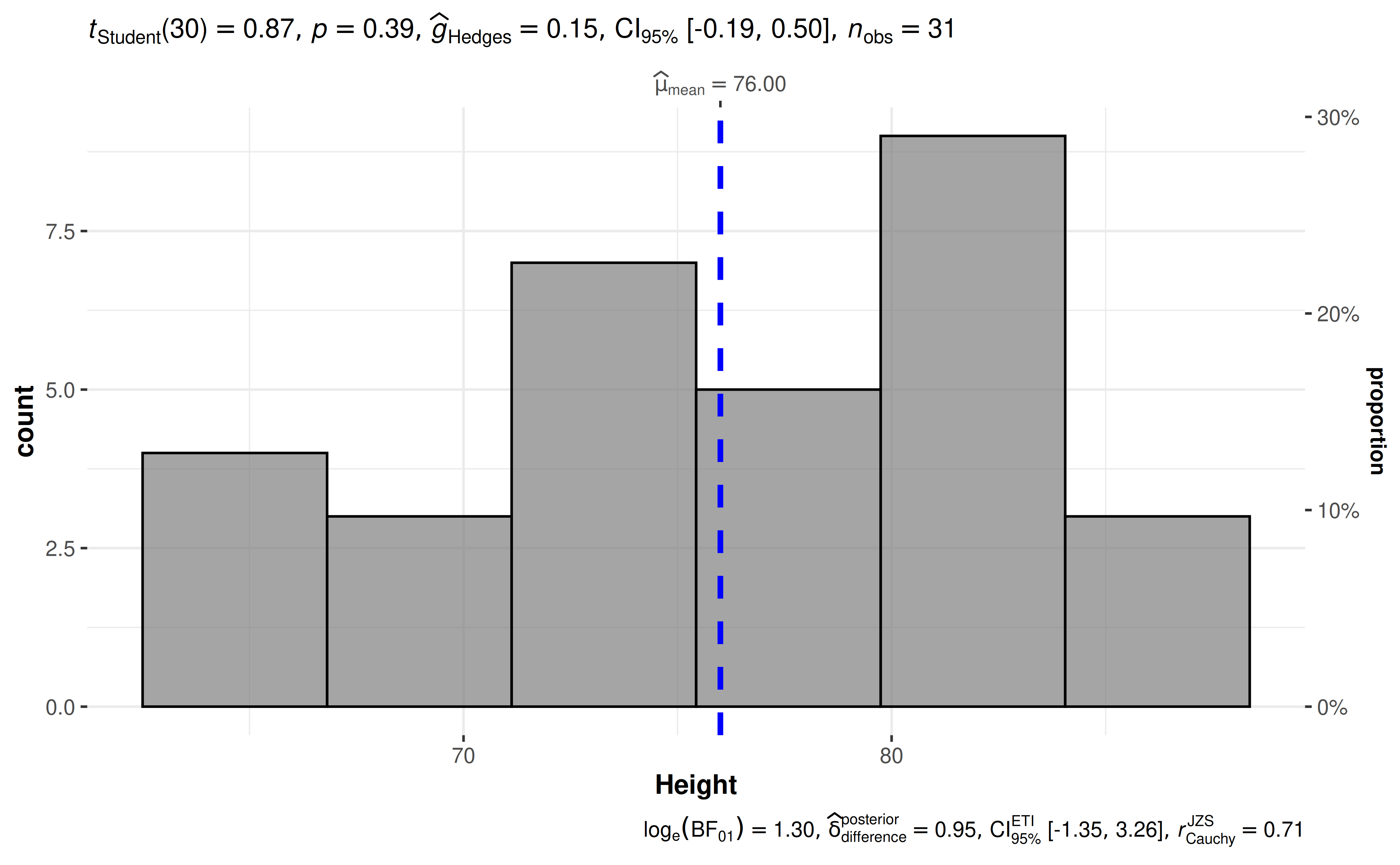

The narrative context (assuming type = "parametric") can complement this plot either as a figure caption or in the main text-

Student’s t-test revealed that, across 31 felled black cherry trees, although the height was higher than expected height of 75 ft., this effect was not statistically significant. The effect size $(g = 0.15)$ was small, as per Cohen’s (1988) conventions. The Bayes Factor for the same analysis revealed that the data were 3.67 times more probable under the null hypothesis as compared to the alternative hypothesis. This can be considered moderate evidence (Jeffreys, 1961) in favor of the null hypothesis.

Suggestions

If you find any bugs or have any suggestions/remarks, please file an issue on GitHub: https://github.com/IndrajeetPatil/ggstatsplot/issues

Citation

You can cite this package/vignette as:

To cite package 'ggstatsplot' in publications use:

  Patil, I. (2021). Visualizations with statistical details: The
  'ggstatsplot' approach. Journal of Open Source Software, 6(61), 3167,
  doi:10.21105/joss.03167

A BibTeX entry for LaTeX users is

  @Article{,
    doi = {10.21105/joss.03167},
    url = {https://doi.org/10.21105/joss.03167},
    year = {2021},
    publisher = {{The Open Journal}},
    volume = {6},
    number = {61},
    pages = {3167},
    author = {Indrajeet Patil},
    title = {{Visualizations with statistical details: The {'ggstatsplot'} approach}},
    journal = {{Journal of Open Source Software}},
  }

gghistostats

Statistical analysis with gghistostats

Grouped analysis with grouped_gghistostats

Grouped analysis with {purrr}