Lifecycle: 
Introduction to ggpiestats
The function ggpiestats can be used for quick
data exploration and/or to prepare
publication-ready pie charts to summarize the
statistical relationship(s) among one or more categorical variables. We
will see examples of how to use this function in this vignette.
To begin with, here are some instances where you would want to use
ggpiestats-
to check if the proportion of observations matches our hypothesized proportion, this is typically known as a “Goodness of Fit” test
to see if the frequency distribution of two categorical variables are independent of each other using the contingency table analysis
to check if the proportion of observations at each level of a categorical variable is equal
ggpiestats works only with data
organized in data frames or tibbles. It will not work with other data
structures like base-R tables or matrices. It can operate on data frames
that are organized with one row per observation or data frames that have
one column containing counts. This vignette provides examples of both
(see examples below).
To help demonstrate how ggpiestats can be used with
categorical (also known as nominal) data, a modified version of the
original Titanic dataset (from the datasets
package) has been provided in the ggstatsplot package
with the name Titanic_full. The Titanic Passenger Survival
Dataset provides information “on the fate of passengers on the fatal
maiden voyage of the ocean liner Titanic, including economic
status (class), sex, age, and survival.”
Let’s have a look at the structure of both.
# looking at the original data in tabular format
dplyr::glimpse(Titanic)
#>  'table' num [1:4, 1:2, 1:2, 1:2] 0 0 35 0 0 0 17 0 118 154 ...
#>  - attr(*, "dimnames")=List of 4
#>   ..$ Class   : chr [1:4] "1st" "2nd" "3rd" "Crew"
#>   ..$ Sex     : chr [1:2] "Male" "Female"
#>   ..$ Age     : chr [1:2] "Child" "Adult"
#>   ..$ Survived: chr [1:2] "No" "Yes"

# looking at the dataset as a tibble or data frame
dplyr::glimpse(Titanic_full)
#> Rows: 2,201
#> Columns: 5
#> $ id       <dbl> 1, 2, 3, 4, 5, 6, 7, 8, 9, 10, 11, 12, 13, 14, 15, 16, 17, 18…
#> $ Class    <ord> 3rd, 3rd, 3rd, 3rd, 3rd, 3rd, 3rd, 3rd, 3rd, 3rd, 3rd, 3rd, 3…
#> $ Sex      <fct> Male, Male, Male, Male, Male, Male, Male, Male, Male, Male, M…
#> $ Age      <fct> Child, Child, Child, Child, Child, Child, Child, Child, Child…
#> $ Survived <fct> No, No, No, No, No, No, No, No, No, No, No, No, No, No, No, N…
Goodness of Fit with ggpiestats
The simplest use case for ggpiestats is that we want to
display information about one categorical or nominal
variable. As part of that display or plot, we may also choose to execute
a chi-squared goodness of fit test to see whether the proportions (or
percentages) in categories of the single variable appear to line up with
our hypothesis or model. To start simple and then expand, let’s say that
we’d like to display a piechart with the percentages of passengers who
did or did not survive. Our initial hypothesis is that it was no
different than flipping a coin. People had a 50/50 chance of
surviving.
ggpiestats(
  data = Titanic_full,
  x = Survived,
  title = "Passenger survival on the Titanic",
  caption = "Source: Titanic survival dataset",
  legend.title = "Survived?"
)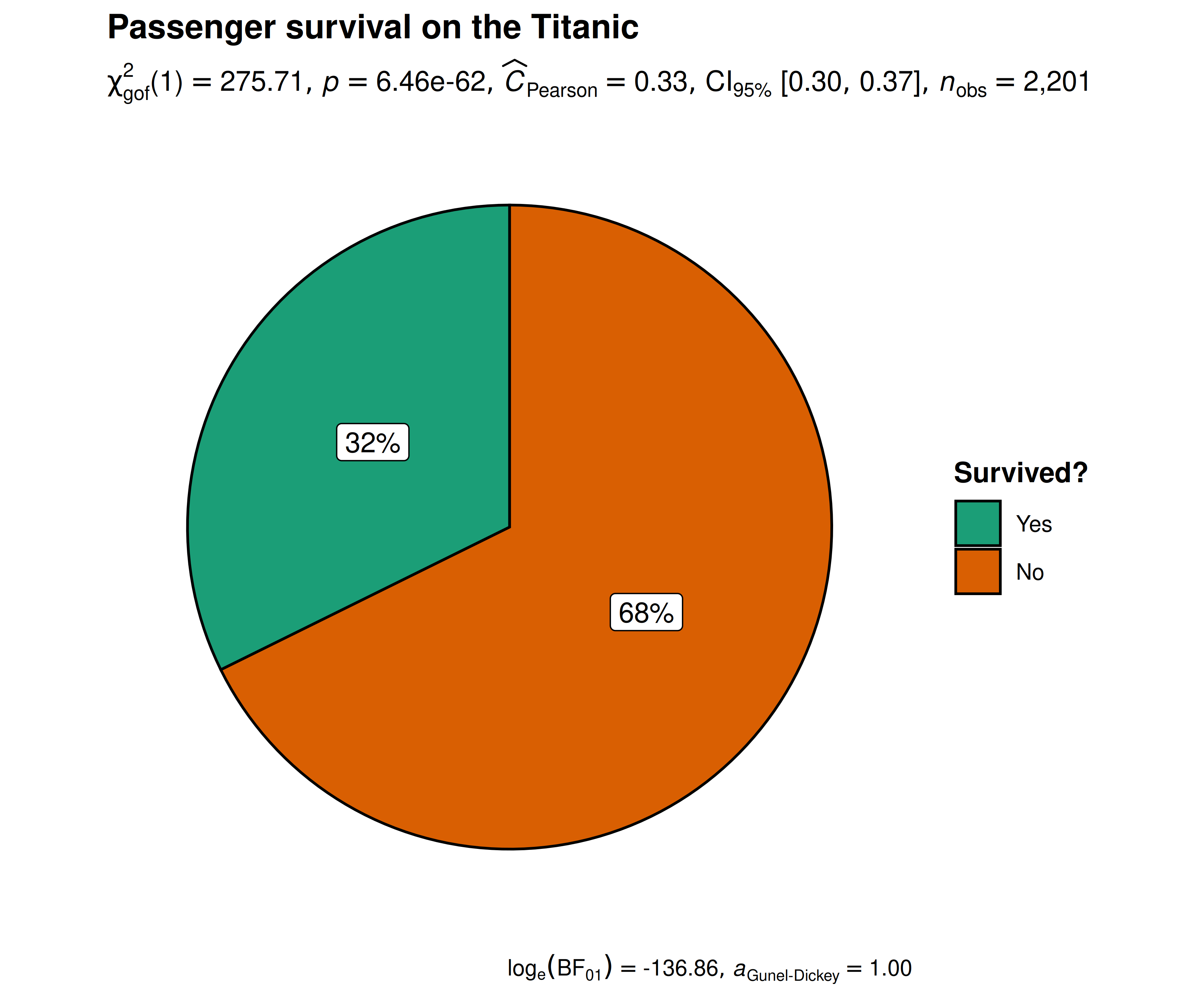
Note: equal proportions per category are the
default, e.g. 50/50, but you can specify any hypothesized ratio you like
with ratio so if our hypothesis was that 80% died and 20%
survived we would add ratio = c(0.80, 0.20) when we entered
the code (the proportions follow the order of the levels of
x).
Independence (or association) with ggpiestats
Let’s next investigate whether the passenger’s sex was independent of, or associated with, their survival status, i.e., we want to test whether the proportion of people who survived was different between the sexes.
ggpiestats(
  data = Titanic_full,
  x = Survived,
  y = Sex
) + # further modification with `{ggplot2}` commands
  ggplot2::theme(
    plot.title = ggplot2::element_text(
      color = "black",
      size = 14,
      hjust = 0
    )
  )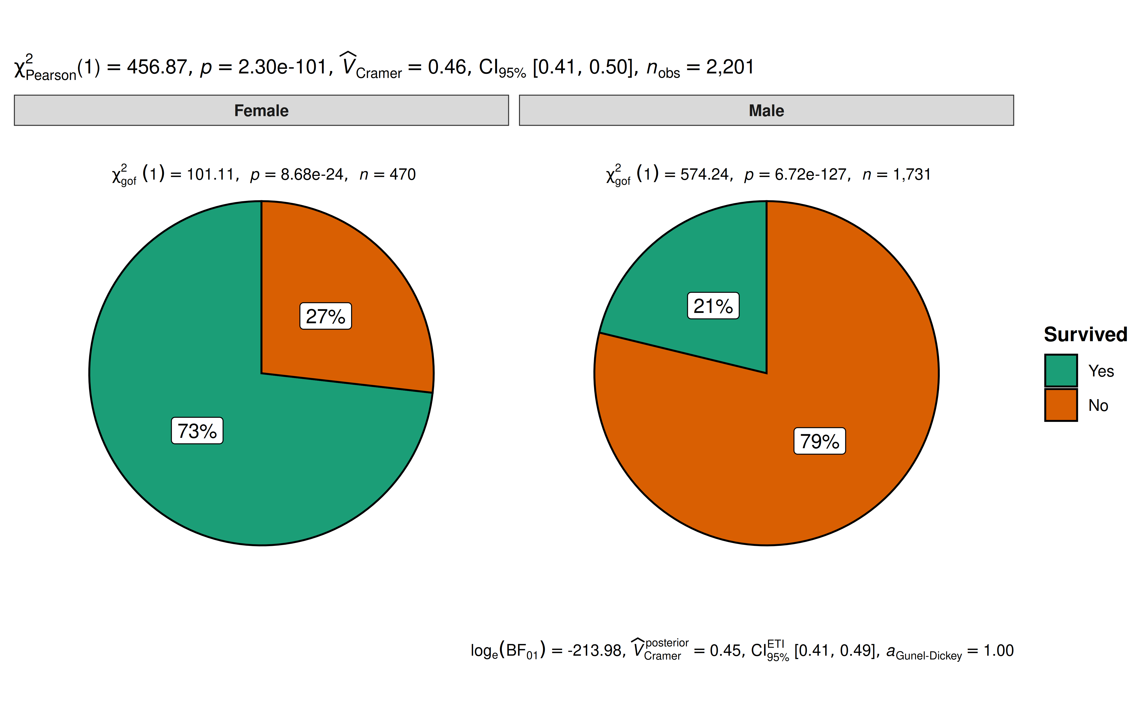
The plot clearly shows that survival rates were very different between males and females. The Pearson’s -test of independence is significant given our large sample size. Additionally, for both females and males, the survival rates were significantly different than 50% as indicated by a goodness of fit test for each gender.
Grouped analysis with grouped_ggpiestats
What if we want to do the same analysis of gender but also factor in the passenger’s age (Age)? We have information that classifies the passengers as Child or Adult, perhaps that makes a difference to their survival rate?
ggstatsplot provides a special helper function for
such instances: grouped_ggpiestats. It is a convenient
wrapper function around combine_plots. It applies
ggpiestats across all levels of a
specified grouping variable and then combines the list
of individual plots into a single plot. Note that the grouping variable
can be anything: conditions in a given study, groups in a study sample,
different studies, etc.
grouped_ggpiestats(
  # arguments relevant for `ggpiestats()`
  data = Titanic_full,
  x = Survived,
  y = Sex,
  grouping.var = Age,
  digits.perc = 1,
  palette = "ggsci::category10_d3",
  # arguments relevant for `combine_plots()`
  annotation.args = list(
    title = "Passenger survival on the Titanic by gender and age",
    caption = "Source: Titanic survival dataset"
  ),
  plotgrid.args = list(nrow = 2L)
)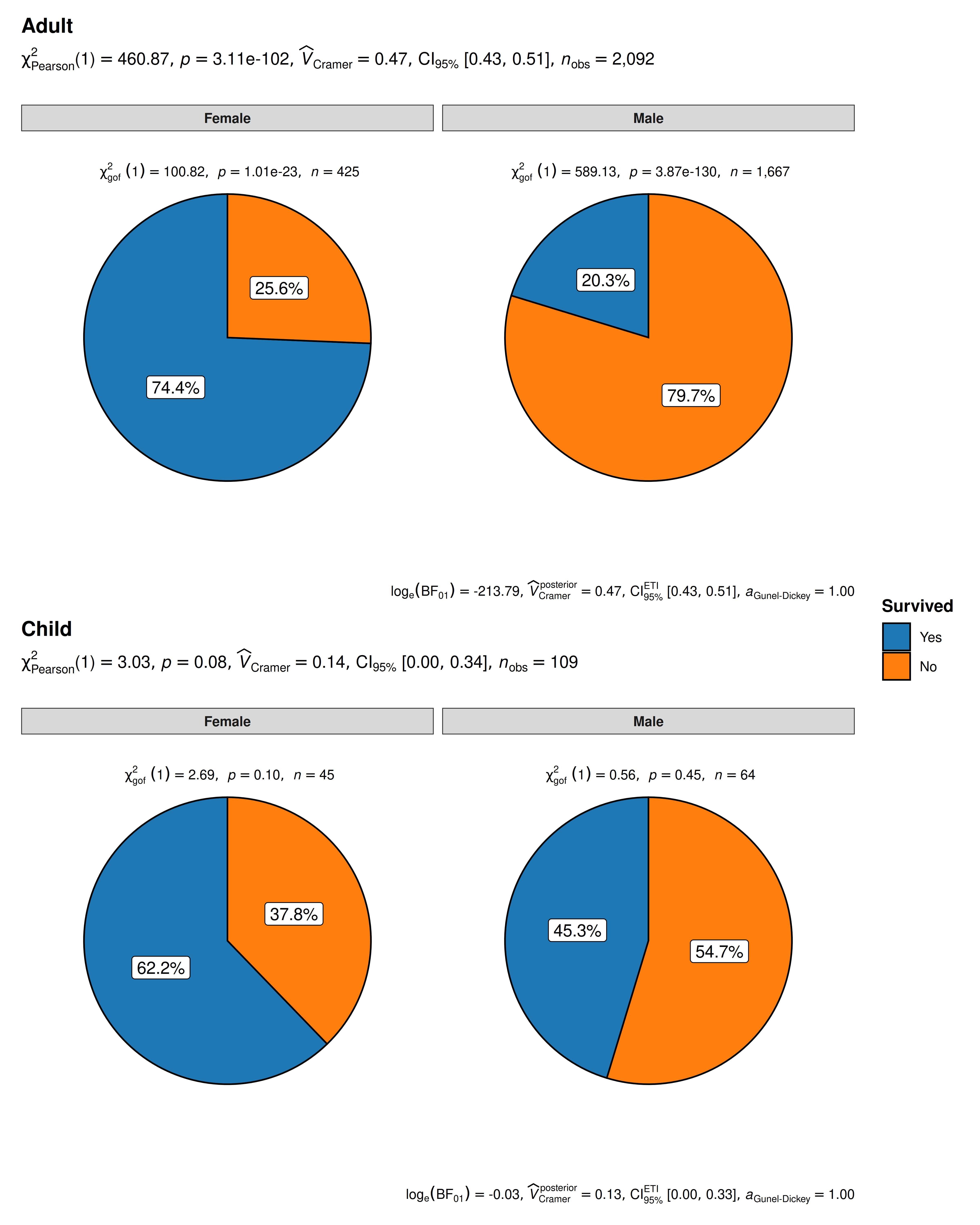
The resulting pie charts and statistics make the story clear. For adults, gender very much matters. Women survived at much higher rates than men. For children, gender is not significantly associated with survival and both male and female children have a survival rate that is not significantly different from 50/50.
Grouped analysis with ggpiestats +
{purrr}
For group-specific arguments or multiple grouping variables, see the programmatic plotting article. It explains how to split the data, customize each call, and combine the resulting plots.
Working with data organized by counts
Use counts when each row contains the frequency of a
combination of categories rather than one observation. See the worked
example with aggregated counts in the bar-chart article; replace
ggbarstats() with ggpiestats() to display the
same analysis as pie charts. Use label = "both" to show
counts and percentages on each slice.
Within-subjects designs
For paired categorical responses, set paired = TRUE to
request McNemar’s test. The variables x and y
must have the same levels. Each row represents one subject or a count of
subjects with a given before/after response.
See the paired-response
example in the bar-chart article. The same call works with
ggpiestats().
Summary of graphics and tests
| graphical element |
geom used |
argument for further modification |
|---|---|---|
| pie slices | ggplot2::geom_col() |
NA |
| labels |
ggplot2::geom_label()/ggrepel::geom_label_repel()
|
label.args |
The statistical tests and effect sizes carried out for each
type are listed in the function documentation: https://www.indrapatil.com/ggstatsplot/reference/ggpiestats.html
Extracting statistical details
Use extract_stats()
to retrieve the statistical results. Both categorical plotting functions
return the same components; see the bar-chart
extraction example for proportion tests and pairwise
comparisons.
Reporting
The bar-chart reporting
example also applies to ggpiestats(): the statistical
analysis is the same, while the graphical representation differs.
Suggestions
If you find any bugs or have any suggestions/remarks, please file an issue on GitHub: https://github.com/IndrajeetPatil/ggstatsplot/issues
Citation
You can cite this package/vignette as:
To cite package 'ggstatsplot' in publications use:

  Patil, I. (2021). Visualizations with statistical details: The
  'ggstatsplot' approach. Journal of Open Source Software, 6(61), 3167,
  doi:10.21105/joss.03167

A BibTeX entry for LaTeX users is

  @Article{,
    doi = {10.21105/joss.03167},
    url = {https://doi.org/10.21105/joss.03167},
    year = {2021},
    publisher = {{The Open Journal}},
    volume = {6},
    number = {61},
    pages = {3167},
    author = {Indrajeet Patil},
    title = {{Visualizations with statistical details: The {'ggstatsplot'} approach}},
    journal = {{Journal of Open Source Software}},
  }